Hello, and welcome! In this post, I'll explain the SSD architecture for object detection, including an overview of the model's structure and which parts have already been implemented.

So, what is SSD?

SSD (Single Shot MultiBox Detector) is an object detection architecture that divides an image into a grid and predicts bounding boxes and class probabilities directly from feature maps at multiple scales. It leverages convolutional layers to extract features and applies predefined anchor boxes of various sizes and aspect ratios at each location, allowing it to efficiently detect objects of different scales. Unlike two-stage detectors, SSD performs detection in a single network pass, making it significantly faster while maintaining competitive accuracy—ideal for real-time applications. That might sound like a lot to take in, but by the end of this post, you’ll have a clearer understanding.

Now, here’s what my model’s structure will look like:

-Model: SSD300
-Base Network: VGG16
-Input Resolution: 300×300
-Feature Maps: 6 scales for multi-scale detection
-Default Boxes: ~8000 per image
-Output: Class scores and box offsets for each default box

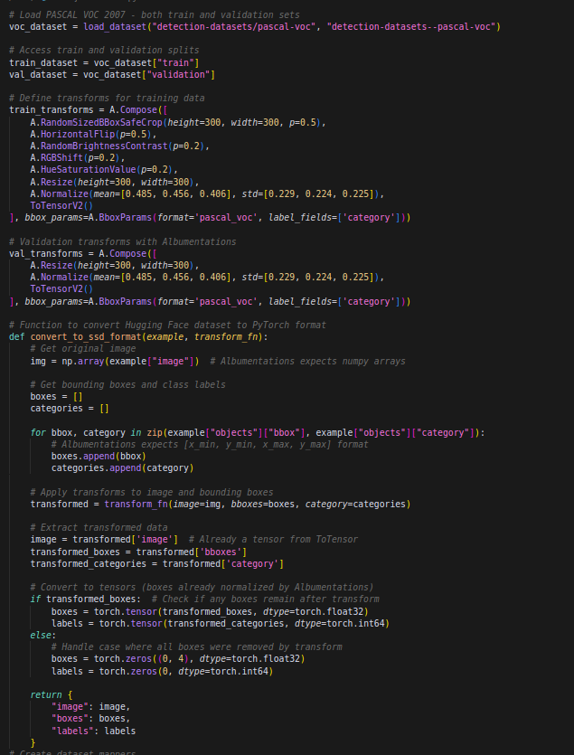
First, I began by loading the dataset for training and validation. For the SSD model, I chose the PASCAL VOC dataset. After that, I applied the necessary transformations and converted the dataset into PyTorch format to ensure compatibility with the training pipeline.

Next, I created a collate function and set up the data loaders.
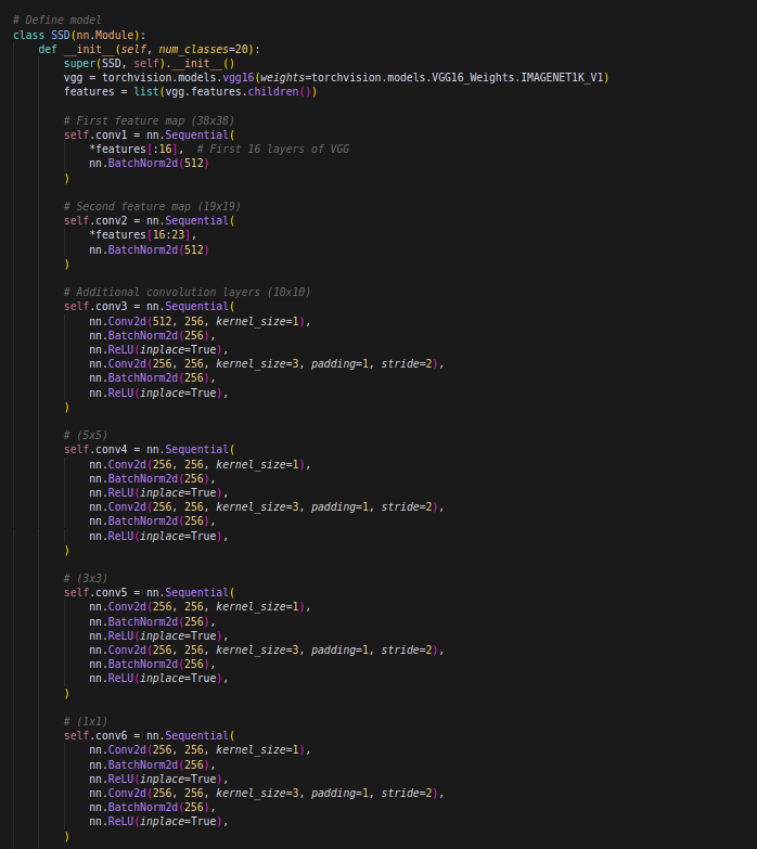
After that, I began working on the actual model definition.

The first step was to load the first and second convolutional layers from a pretrained PASCAL VOC model. This is done to allow the network to leverage learned features, speeding up training and improving generalization. Then, I added four custom convolutional layers to further refine feature extraction for object detection. The convolutional layers have sizes of 38×38, 19×19, 10×10, 5×5, 3×3, and 1×1. Each layer produces a feature map, capturing details from fine-grained features at 38×38 to high-level, larger features at 1×1, enabling the model to detect objects at multiple scales.

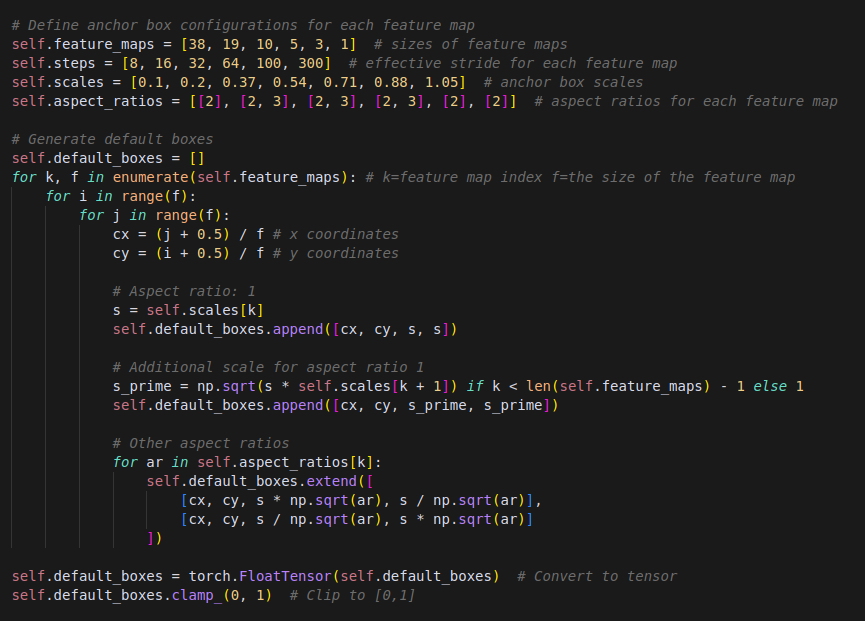
Once a feature map was generated for each convolutional layer, the next step was to add random default anchor boxes at every index of the feature maps. I defined anchor box configurations for each feature map and then created a function with a nested loop. This function iterates through every index in the feature map, traversing its rows and columns to locate the center of each grid cell. It places default boxes of various sizes and aspect ratios surrounding the the center, ensuring robust multi-scale object detection.

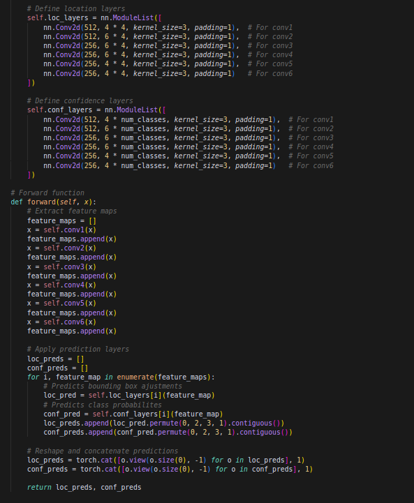
Now, we are ready to predict the bounding box adjustments and class probabilities for the input image. This step is often referred to as the “prediction head”. Within the SSD model, I defined a sequence of convolutional layers responsible for predicting the bounding box offsets and class probabilities for each default box.

In the forward pass, the input image is passed through these convolutional layers, which produce feature maps at different scales. These feature maps are then used to generate predictions for each default box. For each default box, the network predicts two things: the offsets (or adjustments) for the bounding box coordinates and the class probabilities for the object within the box.

This post documents the state of the SSD model as of the 23rd of March, 2025.
To see the current state of the model visit:

SSD object detection model